Estimating the Flow Rate of the
Lowell Glacier
Using ERS Tandem Mode Data
Ian G. Cumming and Joe X. Zhang
Dept. of Electrical and Computer Engineering
The University of British Columbia
2356 Main Mall, Vancouver, B.C.
Canada V6T 1Z4
ianc@ee.ubc.ca, joez@ee.ubc.ca
http://www.ee.ubc.ca/sar/
Abstract
ERS tandem mode differential SAR interferometry (InSAR) has been widely applied to the measurement of displacement or topography of the earth's surface. One interesting example is monitoring the flow of glaciers. In this paper, we resolve the InSAR-measured flow by assuming that the glacier's flow direction is parallel to the surface and to the medial moraine. Both ascending and descending pass data of the Lowell Glacier are processed to obtain the flow rate of the glacier surface. The combination of these two results, along with the assumptions above, can give the 3-D flow rate of the glacier.
1. Introduction
Glaciers are important components of the hydrological cycle in mountainous areas. They are key indicators of climate change, and also are important natural resources that must be monitored and managed. An understanding of the process, which could lead to such change, is hindered by the inability to make accurate measurements of the state of the glaciers. Ground-based measurements are capable of sampling only limited locations at favourable times of the year and the costs of field logistics and personnel are not always affordable. Satellite remote sensing techniques offer the potential for dense and wide-scale monitoring of glaciers at many times of the year. Some research has been done to estimate the surface displacement of glaciers using differential space-borne InSAR techniques [Goldstein:93, Joughin:96, Vachon:96b, Rott:96, Cumming:96].
Interferometric Synthetic Aperture Radar (InSAR) is the process of extracting geophysical information from the phase differences between two or more SAR images. Since Graham [Graham:74] first demonstrated InSAR by using an airborne XTI SAR system in 1974, a lot of interesting research work has been done to examine the potential usefulness of InSAR systems. Major progress has been achieved to make digital elevation models (DEM) of the imaged area of the earth's surface by measuring the phase differences between two registered SAR images, taken with a shift in the viewing angle of the sensor. Accuracies of up to 10 m rms for height measurement over areas of relatively flat, stable terrain has been quoted [Massonnet:93, Askne:93].
In order to estimate the flow rates of glaciers, we need to obtain data with a suitable time interval between the two registered SAR images, then try to separate the phase due to the displacement between the data takes from that due to terrain topography. Sometimes this is not easy to accomplish accurately. Ideally, to get the phase due to the surface displacement only, the viewing angle shift (normal baseline) should strictly be zero and the displacement gradient should be small with respect to the radar wavelength. But this condition is rarely achieved in practice, as baselines are invariably non-zero. However, if the topography information is known, we can still derive the phase part due to surface motion [Vachon:96b].
The time interval between two successive SAR images which cover the same area of the earth's surface is 1, 3, 35 or 165 days for the ERS SARs, but the orbit is not controlled accurately enough to obtain the desired viewing angle for all pairs. Environmental conditions or glacier movements sometimes cause loss of coherence, which can even make registration impossible. So, in order to make accurate measurements of the flow rates of the glaciers, we choose C-band ERS1/ERS2 Tandem Mission data with one-day repeat overage. The potential accuracy of this method can be 4 cm/day rms for the glacier flow rate measurement [Vachon:96b].
In this paper, we select the Lowell Glacier near the border of British Columbia and the Yukon in Canada (N 60.3o W 138.3o) as our research site. We use both ascending and descending data to solve the 3-D flow rate of the glacier under the following assumptions:
2. Experimental Data and Results
The Lowell Glacier is a typical alpine glacier in the Yukon near the British Columbia border. We study an area around 5 km wide and 30 km long, running approximately from the west to the east extending to the terminus of the glacier.
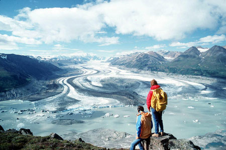
Photo of the terminus of the Lowell Glacier taken from across the Alsek River (courtesy of Parks Canada).
Figure 1 is a descending-pass SAR magnitude image taken on October 23, 1995 that gives an overview of the Lowell Glacier and its surroundings.
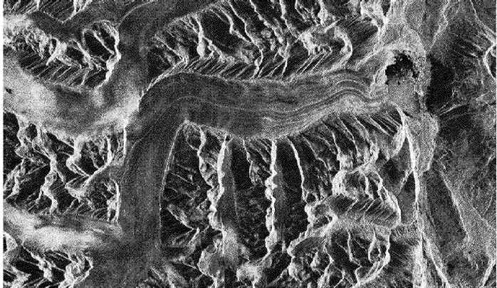
Figure 1 SAR image of the Lowell Glacier, October 23, 1995.
Azimuth: top-to-bottom. Ground range: right-to-left. The scene covers an area of 23x60 km.
In the left part of the scene, the Lowell Glacier flows from the south, then takes a 90o bend, where it momentarily joins with the Dusty Glacier. A medial moraine begins near this point, and runs the remaining length of the Lowell Glacier. Because the upper part of the Lowell Glacier is almost perpendicular to the radar line of sight, we won't be able to estimate the displacement of this part of glacier. In our experiment, we focus on the remaining lower part of the glacier. On the right of the scene, the glacier flows into a terminal moraine and lake, and then the Alsek River.
It is worth noting that there are several distinguishable moraine lines on the surface of the glacier, which show the direction of the surface displacement, assuming the present flow directions have remained stable for a long time. The longest moraine line is close to the glacier centerline. We consider this line as the flow direction of the glacier during our experiment.
The tandem mode passes available and their measured coherence magnitude r are listed in Table 1. The 31/01 Dec/Jan 1995/96 and 22/23 Mar 1996 data are still being processed. In examining the beam geometry and the images, we found that layover is not a problem on the glacier surface in both ascending and descending data. In the case of the ascending pass, the radar line of sight is far from parallel to the glacier flow direction (the angle is 45o). This will lower the measurement accuracy by a small amount.
|
Date of first scene |
RO |
Bn (m) |
r |
Type |
|
Sep 17, 1995 |
300 |
-82 |
0.18 |
Descending |
|
Oct 22, 1995 |
300 |
-87 |
0.73 |
Descending |
|
Dec 31, 1995 |
300 |
135 |
---- |
Descending |
|
Feb 04, 1996 |
300 |
-185 |
0.51 |
Descending |
|
Sep 29, 1995 |
464 |
218 |
0.21 |
Ascending |
|
Jan 12, 1996 |
464 |
-113 |
0.68 |
Ascending |
|
Feb 16, 1996 |
464 |
-169 |
0.62 |
Ascending |
|
Mar 22, 1996 |
464 |
-108 |
---- |
Ascending |
Table 1 Summary of ERS-1/2 passes over the Lowell Glacier.
In order to achieve reasonable estimation accuracy, we require that the scene coherence magnitude be high enough (say, r > 0.4). So we selected the four highest-coherence pairs of data from the above table to continue our experiment. Figures 2 and 3 are representative interferogram maps for descending and ascending scenes.

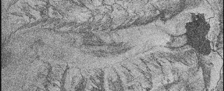

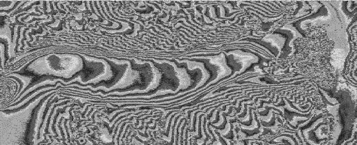
Figure 2 Representative descending pass interferogram from October 22/23, 1995.
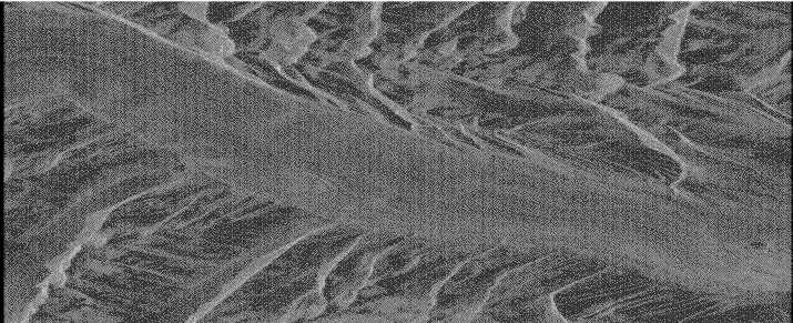
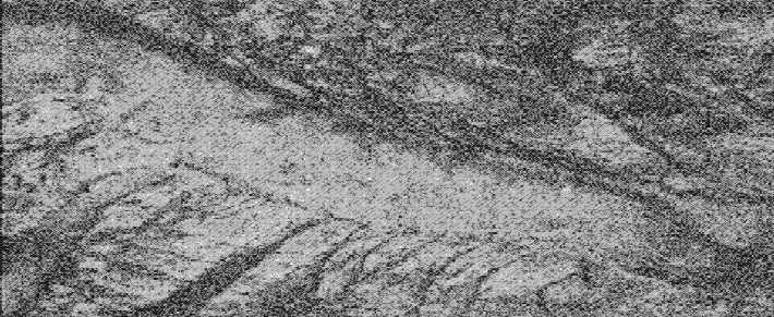

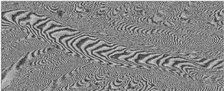
Figure 3 Representative ascending pass interferogram from February 16/17, 1996.
Because no DEM data is available on the Lowell Glacier, we use the 1:50,000 Canada topographic map (115B7-8/115C5) published in 1987. The elevation along the glacier centerline is shown in Figure 4. If the relative elevation accuracy read from the map is 10 m, a relative displacement error of 0.08 cm is made with a 100-m baseline.
Figure 4 Elevation along the glacier centerline.
At the toe of the glacier, we find a rock area and consider the displacement to be zero at this point. After registering the map data to the interferogram, the phase difference can be calculated by subtracting the phase due to topography from the interferogram. Then the phase change is converted to radar line of sight (LOS) displacement. Figures 5 and 6 show the LOS displacement dR along the centerline of the glacier for the descending and ascending passes respectively.
Figure 5 LOS displacement along the glacier centerline derived from the descending pass data
Figure 6 LOS displacement along the glacier centerline derived from the ascending pass data.
From Figures 5 and 6, we observe that the agreement between the measurements taken on the two dates is quite consistent. Without addressing the possibility that the flow rates can change from month to month, or the existence of height errors, this consistency suggests the InSAR-measured LOS measurements can be accurate to about +/- 2 cm/day.
From Figures 5 and 6, we also note the existence of significant
differences in LOS displacement due to the differing viewing angles. We can
take advantage of this difference to check the ``flow parallel to the medial
moraine'' assumption and to compute the 3D flow rates of the glacier. By
using the geometric model of Vachon et al. [Vachon:96a], we can
calculate the glacier surface displacement based on the following
formula:

Figure 7 shows the surface displacement of the glacier obtained from the geometry (1). We can see that results derived from descending pass and ascending pass data agree quite well except near the toe of the glacier. The agreement of the ascending/descending results in the upper glacier testifies to the validity of the flow assumptions in that region. The disagreement near the terminus is likely due to more complex flow patterns in this area of high ablation.
Figure 7 Surface displacement along the glacier centerline.
3. Conclusions
In this paper, we have shown that spaceborne SAR interferometry can be used to estimate the flow rate of the typical high-latitude alpine glacier. We measured a peak flow rate of 50 cm/day on the Lowell Glacier. The combination of ascending and descending passes can help understand the mechanism of the glacier surface movement, if both the ascending and descending pass scenes have high coherence, the glacier flow directions are within 70o of the radar LOS and the assumption of constant flow is valid. We are now processing additional data sets to verify the measurement technique and further check the consistency of results.
Acknowledgments
As part of the Tandem Mission Opportunity, the authors are very grateful to the European Space Agency for the high-quality ERS data. We would like to thank Mr. Mike Seymour of the Radar Remote Sensing Group, UBC, for providing the InSAR programs and helpful discussions and Dr. Wei Xu for the phase unwrapping software. UBC’s NSERC/MacDonald Dettwiler Industrial Research Chair in Radar Remote Sensing has provided funding for the project.
References
[Askne:93] J. Askne and J. O. Hagberg, "Potential of Interferometric SAR for Classification of Land Surfaces", Proc. IGARSS'93, pp. 18-21, August 1993.
[Cumming:96] I. G. Cumming, J.-L. Valero, P. W. Vachon, M. Brugman, K. Mattar, D. Geudtner, M. S. Seymour, and A. L. Gray, "Results of ERS Interferometry Measurements of Alpine Glaciers", in Proc. 18th Ann. Symp. of the Can. Remote Sensing Soc., Vancouver, BC, pp. 324-329, March 25-29, 1996.
[Graham:74] L. C. Graham, "Satellite Interferometer Radar for Topographic Mapping", Proc. IEEE, vol. 62, pp. 763-768, 1974.
[Goldstein:93] R. M. Goldstein, H. Engelhardt, B. Kamb, and R. M. Frolich, "Satellite Radar Interferometry for Monitoring Ice Sheet Motion: Application to an Antarctic Ice Stream", Science, vol. 262, pp. 1525-1530, December 1993.
[Joughin:96] I. Joughin, D. Winebrenner, M. Fahnestock, R. Kwok, and W. Krabill, "Measurement of Ice Sheet Topography Using Satellite Radar Interferometry", J. of Glaciology, vol. 42, pp. 10-22, 1996.
[Massonnet:93] D. Massonnet and T. Rabaute, "Radar Interferometry: Limits and Potential", IEEE Trans. on Geoscience and Remote Sensing, vol. 31, pp. 455-464, March 1993.
[Rott:96] H. Rott and A. Siegel, "Glaciological Studies in the Alps and in Antarctica Using ERS Interferometric SAR", in ESA Workshop on Applications of ERS SAR Interferometry, (http://www.geo.unizh.ch/rsl/fringe96/), University of Zurich, Switzerland, Sept. 1996.
[Vachon:96a] P. W. Vachon, D. Geudtner, A. L. Gray, K. Mattar, M. Brugman, I. G. Cumming, and J. L. Valero, Airborne and Spaceborne SAR Interferometry: Application to the Athabasca Glacier Area, Proc. IGARSS'96, pp. 2255-2257, May 1996.
[Vachon:96b] P. W. Vachon, D. Geudtner, K. Mattar, A. L. Gray, M. Brugman, and I. G. Cumming, "Differential SAR Interferometry Measurements of Athabasca and Saskatchewan Glacier Flow Rate", Canadian J. Remote Sensing, vol. 22, pp. 287-296, September 1996.